Goal: This lecture is dedicated to a classical model in disordered systems: the directed polymer in random media. It has been introduced to model vortices in superconductur or domain wall in magnetic film. We will focus here on the algorithms that identify the ground state or compute the free energy at temperature T, as well as, on the Cole-Hopf transformation that map this model on the KPZ equation.

Polymers, interfaces and manifolds in random media

We consider the following potential energy

E_{pot}=\int dr{\frac {\sigma }{2}}(\nabla h)^{2}+V(r,h)

The first term represents the elasticity of the manifold and the second term is the quenched disorder, due to the impurities. In general, the medium is D-dimensional, the internal coordinate of the manifold is d-dimensional and the height filed is N-dimensional. Hence,the following equations always holds:

D=d+N

In practice, we will study two cases:

Directed Polymers ( $d=1$ ), $D=1+N$ . Examples are vortices, fronts...
Elastic interfaces ( $N=1$ ), $D=d+1$ . Examples are domain walls...

Today we restrict to polymers. Note that they are directed because their configuration $h(r)$ is uni-valuated. It is useful to study the model using the following change of variable

h\to x,\quad r\to t

Directed polymers

Dijkstra Algorithm and transfer matrix

Sketch of the discrete Directed Polymer model. At each time the polymer grows either one step left either one step right. A random energy

V(\tau ,x)

is associated at each node and the total energy is simply

E[x(\tau )]=\sum _{\tau =0}^{t}V(\tau ,x)

.

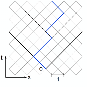
We introduce a lattice model for the directed polymer (see figure). In a companion notebook we provide the implementation of the powerful Dijkstra algorithm.

Dijkstra allows to identify the minimal energy among the exponential number of configurations $x(\tau )$

E_{\min }=\min _{x(\tau )}E[x(\tau )].

We are also interested in the ground state configuration $x_{\min }(\tau )$ . For both quantities we expect scale invariance with two exponents $\theta ,\zeta$ for the energy and for the roughness

E_{\min }=c_{\infty }t+b_{\infty }t^{\theta }\chi ,\quad x_{\min }(t/2))\sim a_{\infty }t^{\zeta }{\tilde {\chi }}

Universal exponents: Both $\theta ,\zeta$ are Independent of the lattice, the disorder distribution, the elastic constants, or the boudanry conditions. Note that $\omega =\theta$ , while for an interface $\omega =d\theta$ .

Non-universal constants: $c_{\infty },b_{\infty },a_{\infty }$ are of order 1 and depend on the lattice, the disorder distribution, the elastic constants... However $c_{\infty }$ is independent on the boudanry conditions!

Universal distributions: $\chi ,{\tilde {\chi }}$ are instead universal, but depends on the boundary condtions. Starting from 2000 a magic connection has been revealed between this model and the smallest eigenvalues of random matrices. In particular I discuss two different boundary conditions:

Droplet: $x(\tau =0)=x(\tau =t)=0$ . In this case, up to rescaling, $\chi$ is distributed as the smallest eigenvalue of a GUE random matrix (Tracy Widom distribution $F_{2}(\chi )$ )

Flat: $x(\tau =0)=0$ while the other end $x(\tau =t)$ is free. In this case, up to rescaling, $\chi$ is distributed as the smallest eigenvalue of a GOE random matrix (Tracy Widom distribution $F_{1}(\chi )$ )

Entropy and scaling relation

It is useful to compute the entropy

{\text{Entropy}}=\ln {\binom {t}{\frac {t-x}{2}}}\approx t\ln 1-{\frac {x^{2}}{t}}+O(x^{4})

From which we infer

\theta =2\zeta -1

Back to the continuum model, a quantuum approach

To fix the idea we can consider polymers of length $t$ , starting in $x_{0}$ and ending in $x$ . We sum over all possible polymers to compute the partition function at temperature $T=1$

Z[x_{t},t;x_{0},0]=\int _{x(0)=x_{0}}^{x(t)=x}{\cal {D}}x\exp \left[-{\frac {1}{T}}\int _{0}^{t}d\tau {\frac {1}{2}}(\partial _{\tau }x)^{2}+V(x,\tau )\right]

The previous equation gives the path integral expression of the propagator for a quantum particle, in the imaginary time. In absence of disorder we have

Z_{\text{free}}[x_{t},t;x_{0},0]={\frac {e^{-x^{2}/(2Tt)}}{\sqrt {2Tt}}}

Note the the potential is a white noise and thus a time dependent potential.

In the spirit of the Feyman Kac formula we write the time-dependent Hamiltonian of the particle

{\hat {H}}=-{\frac {T}{2}}{\frac {d^{2}}{dx^{2}}}+{\frac {1}{T}}V(x,\tau )

The partition function is the solution of the Schrodinger-like equation:

\partial _{t}Z=-{\hat {H}}Z={\frac {T}{2}}{\frac {d^{2}Z}{dx^{2}}}-{\frac {V(x,\tau )}{T}}Z

The initial condition is $Z[x_{t},t=0;x_{0},0]=\delta (x-x_{0})$ . For simplicity, ${\overline {V(x,\tau )V(x',\tau ')}}=D\delta (x-x')\delta (\tau -\tau ')$

DISCUTERE CON SATYA LEGAMI FEYMAN KAC FORMULA / transfer matrix

In this equation the noise is multiplicative and not additive as in the previous lecture. However, all KPZ results can be employed today, thanks to the Cole Hopf transformation.