T-6

Goal: So far we have discussed the equilibrium properties of disordered systems, that are encoded in their partition function/free energy. When a system (following Langevin, Monte Carlo dynamics) equilibrates at sufficiently large times, its long-time properties are captured by these equilibrium calculations. In glassy systems the equilibration timescales are extremely large: for very large timescales the system does not visit equilibrium configurations, but rather metastable states. In this set of problems, we characterize the energy landscape of the spherical $p$-spin by studying its metastable states (local minima).
Techniques: conditional probabilities, saddle point, random matrix theory.

Dynamics, optimization, trapping local minima

Convex and rugged energy landscapes.

• Rugged landscapes. Consider the spherical $p$-spin model: $E({\vec {\sigma }})$ is an energy landscape . It is a random function on configuration space (the surface ${\mathcal {S}}_{N}$ of the sphere). This landscape has its global minimum(a) at the ground state configuration(s): the energy density of the ground state(s) can be obtained studying the partition function $Z$ in the limit $\beta \to \infty$. 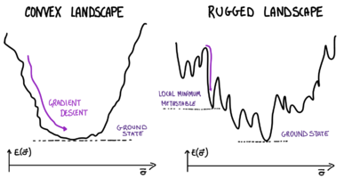Besides the ground state(s), the energy landscape can have other local minima; fully-connected models of glasses are characterized by the fact that there are plenty of these local minima: the energy landscape is rugged, see the sketch.


• Optimization by gradient descent. Suppose that we are interested in finding the configurations of minimal energy, starting from an arbitrary configuration ${\vec {\sigma }}_{0}$: we can implement a dynamics in which we progressively update the configuration moving towards lower and lower values of the energy, hoping to eventually converge to the ground state(s). The simplest dynamics of this sort is gradient descent, ${\frac {d{\vec {\sigma }}(t)}{dt}}=-\nabla _{\perp }E({\vec {\sigma }})$

  where $\nabla _{\perp }E({\vec {\sigma }})$ is the gradient of the landscape restricted to the sphere. The dynamics stops when it reaches a stationary point , a configuration where $\nabla _{\perp }E({\vec {\sigma }})=0$. If the landscape has a convex structure, this will be the ground state; if the energy landscape is very non-convex like in glasses, the end point of this algorithm will be a local minimum at energies much higher than the ground state (see sketch).



• Stationary points and complexity. To guess where gradient descent dynamics (or Langevin dynamics ) are expected to converge, it is useful to understand the distribution of the stationary points, i.e. the number ${\mathcal {N}}(\epsilon )$ of such configuration having a given energy density $\epsilon$. In fully-connected models, this quantity has an exponential scaling, ${\mathcal {N}}(\epsilon )\sim {\text{exp}}\left(N\Sigma (\epsilon )\right)$, where $\Sigma (\epsilon )$ is the landscape’s complexity. ^[*] . Stationary points can be stable (local minima), or unstable (saddles or local maxima): their stability is encoded in the spectrum of the Hessian matrix $\nabla _{\perp }^{2}E({\vec {\sigma }})$: when all the eigenvalues of the Hessian are positive, the point is a local minimum (and a saddle otherwise).

[*] - This quantity looks similar to the entropy $S(\epsilon )$ we computed for the REM in Problem 1. However, while the entropy counts all configurations at a given energy density, the complexity $\Sigma (\epsilon )$ accounts only for the stationary points.

Problems

In these problems, we discuss the computation of the annealed complexity of the spherical $p$-spin model, which is defined by

$\Sigma _{\text{a}}(\epsilon )=\lim _{N\to \infty }{\frac {1}{N}}\log {\overline {{\mathcal {N}}(\epsilon )}},\quad \quad {\mathcal {N}}(\epsilon )=\left\{{\text{number stat. points of energy density }}\epsilon \right\}$

Problem 5.1: the Kac-Rice formula and the complexity

1. The Kac-Rice formula. Consider first a random function of one variable $f(x)$ defined on an interval $[a,b]$, and let ${\mathcal {N}}$ be the number of points $x$ such that $f(x)=0$. Justify why

   ${\overline {\mathcal {N}}}=\int _{a}^{b}dx\,p_{0}(x),\quad \quad p_{0}(x)={\overline {\delta (f(x))|f'(x)|}}$

   where $p_{0}(x)$ is the probability density that $x$ is a zero of the function. In particular, why is the derivative of the function appearing in this formula? Consider now the number of stationary points ${\mathcal {N}}(\epsilon )$ of the $p$-spin energy landscape, which satisfy $\nabla _{\perp }E({\vec {\sigma }})=0$. Justify why the generalization of the formula above gives

   ${\overline {{\mathcal {N}}(\epsilon )}}=\int _{{\mathcal {S}}_{N}}d{\vec {\sigma }}\,p_{\epsilon }({\vec {\sigma }}),\quad \quad p_{\epsilon }({\vec {\sigma }})={\overline {|{\text{det}}\nabla _{\perp }^{2}E({\vec {\sigma }})|\,\,\delta (\nabla _{\perp }E({\vec {\sigma }})=0)\,\,\delta (E({\vec {\sigma }})-N\epsilon )}}$

   where $p_{\epsilon }({\vec {\sigma }})$ is the probability density that ${\vec {\sigma }}$ is a stationary point of energy density $\epsilon$, and $\nabla _{\perp }^{2}E({\vec {\sigma }})$ is the Hessian matrix of the function $E({\vec {\sigma }})$ restricted to the sphere.

2. Statistical rotational invariance. Recall the expression of the correlations of the energy landscape of the $p$-spin computed in Problem 3.1: in which sense the correlation function is rotationally invariant? Justify why rotational invariance implies that

   ${\overline {{\mathcal {N}}(\epsilon )}}=(2\pi e)^{\frac {N}{2}}\,p_{\epsilon }({\vec {1}})$

   where ${\vec {1}}=(1,1,1,\cdots ,1)$ is one fixed vector belonging to the surface of the sphere. Where does the prefactor arise from?

3. Gaussianity and correlations.
   • Determine the distribution of the quantity $E({\vec {1}})$.
   • The entries of $\nabla _{\perp }E({\vec {1}}),\nabla _{\perp }^{2}E({\vec {1}})$ are Gaussian variables. One can show that the $N-1$ components of $\nabla _{\perp }E({\vec {1}})$ are uncorrelated to $E({\vec {1}}),\nabla _{\perp }^{2}E({\vec {1}})$; they have zero mean and covariances ${\overline {(\nabla _{\perp }E)_{\alpha }\,(\nabla _{\perp }E)_{\beta }}}=p\,\delta _{\alpha \beta }+O\left({\frac {1}{N}}\right).$ Compute the probability density that $\nabla _{\perp }E({\vec {1}})=0$.
   • The $(N-1)\times (N-1)$ matrix $\nabla _{\perp }^{2}E({\vec {\sigma }})$ conditioned to the fact that $E({\vec {1}})=N\epsilon$ can be written as

     $[\nabla _{\perp }^{2}E({\vec {1}})]_{\alpha \beta }=M_{\alpha \beta }-p\epsilon \,\delta _{\alpha \beta },$

     where the matrix $M$ has random entries with zero average and correlations ${\overline {{M}_{\alpha \beta }\,{M}_{\gamma \delta }}}={\frac {p(p-1)}{N}}\left(\delta _{\alpha \gamma }\delta _{\beta \delta }+\delta _{\alpha \delta }\delta _{\beta \gamma }\right)$ Combining this with the results above, show that

     ${\overline {{\mathcal {N}}(\epsilon )}}=(2\pi e)^{\frac {N}{2}}\,{\frac {1}{(2\pi \,p)^{\frac {N-1}{2}}}}\;{\sqrt {\frac {N}{2\pi }}}e^{-{\frac {N\epsilon ^{2}}{2}}}\;{\overline {|{\text{det}}\left(M-p\epsilon \mathbb {I} \right)|}}$

Problem 5.2: the Hessian and random matrix theory

To get the complexity, it remains to compute the expectation value of the determinant of the Hessian matrix: this is the goal of this problem. We will do this exploiting results from random matrix theory.

1. Gaussian Random matrices. Show that the matrix $M$ is a GOE matrix, i.e. a matrix taken from the Gaussian Orthogonal Ensemble, meaning that it is a symmetric matrix with distribution $P(M)=Z_{N}^{-1}e^{-{\frac {N}{4\sigma ^{2}}}{\text{Tr}}M^{2}}.$ What is the value of $\sigma ^{2}$?

2. Eigenvalue density and concentration. Let $\lambda _{\alpha }$ be the eigenvalues of the matrix $M$. Show that the following identity holds:

   ${\overline {|{\text{det}}\left(M-p\epsilon \mathbb {I} \right)|}}={\overline {{\text{exp}}\left[(N-1)\left(\int d\lambda \,\rho _{N}(\lambda )\,\log |\lambda -p\epsilon |\right)\right]}},\quad \quad \rho _{N}(\lambda )={\frac {1}{N-1}}\sum _{\alpha =1}^{N-1}\delta (\lambda -\lambda _{\alpha })$

   where $\rho _{N}(\lambda )$ is the empirical eigenvalue density. It can be shown that if $M$ is a GOE matrix, the distribution of the empirical density has a large deviation form (recall TD1) with speed $N^{2}$, meaning that $P_{N}[\rho ]=e^{-N^{2}\,g[\rho ]}$ where now $g[\cdot ]$ is a functional (a function of a function). Using a saddle point argument, show that this implies

   ${\overline {{\text{exp}}\left[(N-1)\left(\int d\lambda \,\rho _{N}(\lambda )\,\log |\lambda -p\epsilon |\right)\right]}}={\text{exp}}\left[N\left(\int d\lambda \,\rho _{\text{typ}}(\lambda +p\epsilon )\,\log |\lambda |\right)+o(N)\right]$

   where $\rho _{\text{typ}}(\lambda )$ is the typical value of the eigenvalue density, which satisfies $g[\rho _{\text{typ}}]=0$.

3. The semicircle and the complexity. The eigenvalue density of GOE matrices is self-averaging, and it equals to

   $\lim _{N\to \infty }\rho _{N}(\lambda )=\lim _{N\to \infty }{\overline {\rho _{N}}}(\lambda )=\rho _{\text{typ}}(\lambda )={\frac {1}{2\pi \sigma ^{2}}}{\sqrt {4\sigma ^{2}-\lambda ^{2}}}$

   • Check this numerically: generate matrices for various values of $N$, plot their empirical eigenvalue density and compare with the asymptotic curve. Is the convergence faster in the bulk, or in the edges of the eigenvalue density, where it vanishes?
   • Combining all the results, show that the annealed complexity is $\Sigma _{\text{a}}(\epsilon )={\frac {1}{2}}\log[4e(p-1)]-{\frac {\epsilon ^{2}}{2}}+I_{p}(\epsilon ),\quad \quad I_{p}(\epsilon )={\frac {2}{\pi }}\int dx{\sqrt {1-\left(x-{\frac {\epsilon }{\epsilon _{\text{th}}}}\right)^{2}}}\,\log |x|,\quad \quad \epsilon _{\text{th}}=-2{\sqrt {\frac {p-1}{p}}}.$

     The integral $I_{p}(\epsilon )$ can be computed explicitly, and one finds:

     $I_{p}(\epsilon )={\begin{cases}&{\frac {\epsilon ^{2}}{\epsilon _{\text{th}}^{2}}}-{\frac {1}{2}}-{\frac {\epsilon }{\epsilon _{\text{th}}}}{\sqrt {{\frac {\epsilon ^{2}}{\epsilon _{\text{th}}^{2}}}-1}}+\log \left({\frac {\epsilon }{\epsilon _{\text{th}}}}+{\sqrt {{\frac {\epsilon ^{2}}{\epsilon _{\text{th}}^{2}}}-1}}\right)-\log 2\quad {\text{if}}\quad \epsilon \leq \epsilon _{\text{th}}\\&{\frac {\epsilon ^{2}}{\epsilon _{\text{th}}^{2}}}-{\frac {1}{2}}-\log 2\quad {\text{if}}\quad \epsilon >\epsilon _{\text{th}}\end{cases}}$

     Plot the annealed complexity, and determine numerically where it vanishes: why is this a lower bound or the ground state energy density?

4. The threshold and the stability. Sketch $\rho _{\text{typ}}(\lambda +p\epsilon )$ for different values of $\epsilon$; recalling that the Hessian encodes for the stability of the stationary points, show that there is a transition in the stability of the stationary points at the critical value of the energy density $\epsilon _{\text{th}}=-2{\sqrt {(p-1)/p}}.$ When are the critical points stable local minima? When are they saddles? Why the stationary points at $\epsilon =\epsilon _{\text{th}}$ are called marginally stable ?

Check out: key concepts

Gradient descent, rugged landscapes, metastable states, Hessian matrices, random matrix theory, landscape’s complexity.