T-7

Goal: The goal of these problems is to understand some features of glassy dynamics (power laws, aging) in a simplified single particle description, the so called trap model.
Techniques: extreme value statistics, asymptotic analysis.

A dynamical dictionary: energy barriers, out-of-equilibrium, aging

Fig 7.1 - Activated jump across an energy barrier.

• Noise and Langevin dynamics. In problems 5 and 6 we have characterized the energy landscape of the spherical $p$-spin, and showed that it is made by plenty of stationary points where gradient descent gets stuck. In presence of noise, ${\frac {d{\vec {\sigma }}(t)}{dt}}=-\nabla _{\perp }E({\vec {\sigma }})+{\vec {\eta }}(t),\quad \quad \langle \eta _{i}(t)\eta _{j}(t')\rangle =2T\delta _{ij}\delta (t-t')$

  the random terms kick the systems in random directions in configuration space, allowing to escape from stationary points. In Langevin dynamics, ${\vec {\eta }}(t)$ a Gaussian vector at each time $t$, uncorrelated from the vectors at other times $t'\neq t$, with zero average and some constant variance proportional to temperature.



• Activation and Arrhenius law. When the noise in the Langevin dynamics is weak (temperature is small), the dynamics does not get stuck in local minima forever, but for very large time. This time depends crucially on the energy barrier which separate the minimum from the other configurations (see Fig 6.1). The Arrhenius law states that the typical timescale $\tau$ required to escape from a local minimum through a barrier of height $\Delta E$ with thermal dynamics with inverse temperature $\beta$ scales as $\tau \sim \tau _{0}e^{-\beta \,\Delta E}$. A dynamics made of jumps from minimum to minimum through the crossing of energy barriers is called activated .



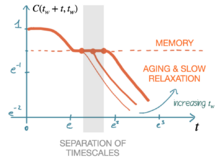
Fig 7.2 - Behaviour of the correlation function in a system displaying aging.
• Equilibrating dynamics. A system evolving with thermal dynamics (e.g. Langevin dynamics) equilibrates dynamically if there is a timescale $\tau _{\text{eq}}$ beyond which the dynamical trajectories sample the configurations of the system ${\vec {\sigma }}$ with the frequency that is prescribed by the Gibbs Boltzmann measure, $\sim e^{-\beta E({\vec {\sigma }})}$, where $\beta$ is the inverse temperature associated to the noise. At equilibrium, one-point functions in time, like the energy of the system, reach a stationary value (the equilibrium value predicted by thermodynamics at that temperature), while two-point functions like the correlation function

  $C(t_{w}+t,t_{w})={\frac {1}{N}}\sum _{i=1}^{N}\sigma _{i}(t_{w})\sigma _{i}(t_{w}+t)$

  are time-translation invariant, meaning that $C(t_{w}+t,t_{w})\sim c(t)$ is only a function of the difference between the two times, and does not depend on $t_{w}$.


• Out-of-equilibrium and aging. In some systems the equilibration timescale $\tau _{\text{eq}}$ is extremely large/diverging with some parameter of the model (like $N$), and for very large time-scales the dynamics is out-of-equilibrium . In glassy systems, out-of-equilibrium dynamics is often characterized by aging: the relaxation timescale of a system (how slow the system evolves) depends on the age of the system itself (on how long the system has evolved so far). Aging can be seen in the behaviour of correlation function, see Fig 7.2: the timescale that the system needs to leave the plateau increases with the age of the system $t_{w}$, meaning that the system is becoming more and more slow as it gets more and more old.



Problems

In the first of these problems, we discuss the main features of the trap model, a model for glassy dynamics. In the second problem, we discuss the interpretation of the model, using what we know about the energy landscape of the REM and spherical $p$-spin models.

Problem 7.1: a simple model for aging


Fig 6.3 - Traps in the trap model.

The trap model is an abstract model for the dynamics in complex landscapes introduced in ^[1] . The configuration space is a collection of $M\gg 1$ traps labeled by $\alpha$ having random depths/energies (see sketch). The dynamics is a sequence of jumps between the traps: the system spends in a trap $\alpha$ an exponentially large time with average $\tau _{\alpha }$ (the probability to jump out of the trap in time $[t,t+dt]$ is $dt/\tau _{\alpha }$.). When the system exits the trap, it jumps into another one randomly chosen among the $M$. The average times are distributed as

$P_{\mu }(\tau )={\frac {\mu \tau _{0}^{\mu }}{\tau ^{1+\mu }}}\quad \quad \tau \geq \tau _{0}$

where $\mu$ is a parameter. In this exercise, we aim at understanding the main features of this dynamics.





1. Condensation and ergodicity breaking. Compute the average trapping time (averaging between the traps) and show that there is a critical value of $\mu$ below which it diverges, signalling a non-ergodic phase (the system needs infinite time to explore the whole configuration space). Consider a dynamics running from time $t_{w}$ to some later time $t_{w}+t$: compute the typical value of the maximal trapping time $\tau _{\text{max}}(t)$ encountered in this time interval, assuming that the system has spent exactly a time $\tau _{\alpha }$ in each visited trap $\alpha$. Show that in the non-ergodic phase $\tau _{\text{max}}(t)\sim t$. Why is this interpretable as a condensation phenomenon?


2. Correlations: slow dynamics and aging. Assume now that the trap represent a collection of microscopic configurations having self overlap $q_{EA}$. Assume that the overlap between configurations of different traps is $q_{0}$. Justify why the correlation function can be written as

   $C(t_{w}+t,t_{w})=q_{EA}\Pi (t,t_{w})+q_{0}\left(1-\Pi (t,t_{w})\right),\quad \quad \Pi (t,t_{w})={\text{probability that systems has not jumped in }}[t_{w},t_{w}+t].$

   In the non-ergodic regime, one finds:

   $\Pi (t,t_{w})={\frac {\sin(\pi \mu )}{\pi }}\int _{\frac {t}{t+t_{w}}}^{1}du(1-u)^{\mu -1}u^{-\mu }.$

   Why is this an indication of aging? Study the asymptotic behaviour of the correlation function for $t\ll t_{w}$ and $t\gg t_{w}$ and show that the dynamics is slow, characterized by power laws. Show that

   $\lim _{t\to \infty }C(t_{w}+t,t_{w})=q_{0}\quad {\text{ for finite }}t_{w},\quad \quad \lim _{t_{w}\to \infty }C(t_{w}+t,t_{w})=q_{EA}\quad {\text{ for finite }}t$ When $q_{0}=0$, this behaviour is called "weak ergodicity breaking".




Problem 7.2: from landscapes to traps

In this exercise, we aim at understanding why the trap model is a good effective model for the exploration of the energy landscape of two models that we have studied so far: the REM and spherical $p$-spin model. While for the $p$-spin we think about Langevin dynamics, for the REM we consider Monte Carlo dynamics: at each time step the system in a given configuration ${\vec {\sigma }}$ with energy $E_{1}$ tries to transition to another configuration that differs with respect to the previous one by a single spin flip; let the energy of this second configuration be $E_{2}$. The transition occurs with probability one if $E_{2}<E_{1}$, and with probability $e^{-\beta (E_{2}-E_{1})}$ otherwise.





1. REM: the golf course landscape. In the REM, the smallest energies values $E_{\alpha }$ among the $M=2^{N}$ can be assumed to be distributed as

   $P_{N}^{\text{extrm}}(E)\approx C_{N}{\text{exp}}\left[{\sqrt {2\log 2}}(E+N{\sqrt {2\log 2}})\right],\quad \quad E<0,\quad \quad C_{N}{\text{ normalization}}$

   Justify the form of this distribution (Hint: recall the discussion on extreme value statistics in Lecture 1!). Consider now one of these deep configurations of energy close to that of the ground state: what is the minimal energy among the $N$ neighbouring configurations, which differs from the previous one by a spin flip? Does it depend on the energy of the original one? Why is this consistent with the results on the entropy of the REM that we computed in Problem 1?


2. REM: trapping times. The results above show that the energy landscape of the REM has a "golf course" structure: configuration with deep energy are isolated, surrounded by configurations of much higher energy (zero energy density). The Arrhenius law states that the time needed for the system to escape from a trap of energy density $\epsilon <0$ and reach a configuration of zero energy density is $\tau \sim e^{-\beta N\epsilon }$. This is a trapping time. Given the energy distribution $P_{N}^{\text{extrm}}(E)$, determine the distribution of trapping times $P_{\mu }(\tau )$: what plays the role of $\mu$?


3. p-spin and the “trap” picture. In Problems 5, we have seen that the energy landscape of the spherical $p$-spin is characterized by the threshold energy, below which plenty of minima appear. Explain why the trap model corresponds to the following picture for the dynamics: the system is trapped into minima below the threshold for exponentially large times, and then jumps from minimum to minimum passing through the threshold energy.




Check out: key concepts

Aging, activation, time-translation invariance, out-of equilibrium dynamics, power laws, decorrelation, condensation, extreme values statistics (typical values of minima).

To know more

• Bouchaud. Weak ergodicity breaking and aging in disordered systems [1]
• Biroli. A crash course on aging [2]
• Kurchan. Six out-of-equilibrium lectures [3]