Introduction: Interfaces and Directed Polymers
The physical properties of many materials are governed by manifolds embedded in them. Examples include: dislocations in crystals, domain walls in ferromagnets or vortex lines in superconductors. We fix the following notation:
-  : spatial dimension of the embedding medium
–
: spatial dimension of the embedding medium
–  : internal dimension of the manifold
–
: internal dimension of the manifold
–  : dimension of the displacement (or height) field
These satisfy the relation:

We focus on two important cases:
Directed Polymers (d = 1)
The configuration is described by a vector function:
 ,
where
,
where  is the internal coordinate. The polymer lives in
  dimensions.
Examples: vortex lines, DNA strands, fronts.
Although polymers may form loops, we restrict to directed polymers, i.e., configurations without overhangs or backward turns.
Interfaces (N = 1)
The interface is described by a scalar height field:
 ,
where
,
where  is the internal coordinate and represents time.
Examples: domain walls and propagating fronts
Again we neglect overhangs or pinch-off: is single-valued
Note that using our notation the 1D front is both an interface and a directed polymer
Directed Polymers on a lattice
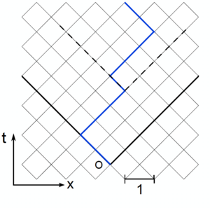
Sketch of the discrete Directed Polymer model. At each time the polymer grows either one step left either one step right. A random energy

is associated at each node and the total energy is simply
![{\displaystyle E[x(\tau )]=\sum _{\tau =0}^{t}V(\tau ,x)}](https://wikimedia.org/api/rest_v1/media/math/render/svg/93b0356dd1c49f25c798e141e27a40d486be2bfe)
.
We introduce a lattice model for the directed polymer (see figure). In a companion notebook we provide the implementation of the powerful Dijkstra algorithm. Dijkstra allows to identify the minimal energy among the exponential number of configurations 
![{\displaystyle E_{\min }=\min _{x(\tau )}E[x(\tau )].}](https://wikimedia.org/api/rest_v1/media/math/render/svg/ad4cafbe3be352ced3ba5e55c5236b8c4444833f)
We are also interested in the ground state configuration  .
For both quantities we expect scale invariance with two exponents
.
For both quantities we expect scale invariance with two exponents  for the energy and for the roughness

Universal exponents: Both are Independent of the lattice, the disorder distribution, the elastic constants, or the boudanry conditions.
Non-universal constants:  are of order 1 and depend on the lattice, the disorder distribution, the elastic constants... However
  is independent on the boudanry conditions!
Universal distributions:  are instead universal, but depends on the boundary condtions. Starting from 2000 a magic connection has been revealed between this model and the smallest eigenvalues of random matrices. In particular I discuss two different boundary conditions:
- Droplet:
 . In this case, up to rescaling,
  is distributed as the smallest eigenvalue of a GUE random matrix (Tracy Widom distribution
  )
)
- Flat:
 while the other end
  is free. In this case, up to rescaling, is distributed as the smallest eigenvalue of a GOE random matrix (Tracy Widom distribution
  )
)
Entropy and scaling relation
It is useful to compute the entropy

From which one could guess from dimensional analysis

This relation is actually exact also for the continuum model.
Directed polymers in the continuum
We now reanalyze the previous problem in the presence of quenched disorder.
Instead of discussing the case of interfaces, we will focus on directed polymers.
Let us consider polymers of length .
The energy associated with a given polymer configuration can be written as
![{\displaystyle E[x(\tau )]=\int _{0}^{t}d\tau \,\left[{\frac {1}{2}}\left({\frac {dx}{d\tau }}\right)^{2}+V(x(\tau ),\tau )\right]}](https://wikimedia.org/api/rest_v1/media/math/render/svg/6c41651a12e1b6cf95ceadfdca1dd70c7097baaa)
The first term describes the elastic energy of the polymer,
while the second one is the disordered potential, which we assume to be

where 'D' is the disorder strength.
Polymer partition function and propagator of a quantum particle
Let us consider polymers starting in  , ending in
  and at thermal equilibrium at temperature
  . The partition function of the model writes as
![{\displaystyle Z(x,t)=\int _{x(0)=0}^{x(t)=x}{\cal {D}}x(\tau )\exp \left[-{\frac {1}{T}}\int _{0}^{t}d\tau {\frac {1}{2}}(\partial _{\tau }x)^{2}+V(x(\tau ),\tau )\right]}](https://wikimedia.org/api/rest_v1/media/math/render/svg/6be96d05745484d7b16302f05367c4eb5d7e577a)
Here, the partition function is written as a sum over all possible paths, corresponding to all possible polymer configurations that start at and end at , weighted by the appropriate Boltzmann factor.
Let's perform the following change of variables:  . We also identifies with
  and
and  as the time.
![{\displaystyle Z(x,{\tilde {t}})=\int _{x(0)=0}^{x({\tilde {t}})=x}{\cal {D}}x(t')\exp \left[{\frac {i}{\hbar }}\int _{0}^{\tilde {t}}dt'{\frac {1}{2}}(\partial _{t'}x)^{2}-V(x(t'),t')\right]}](https://wikimedia.org/api/rest_v1/media/math/render/svg/fbe30988e17e8a07bb2f0ed0dc15d77bbafa04be)
Note that ![{\displaystyle S[x]=\int _{0}^{\tilde {t}}dt'{\frac {1}{2}}(\partial _{t'}x)^{2}-V(x(t'),t')}](https://wikimedia.org/api/rest_v1/media/math/render/svg/24e6431964c1d024dccfd9c0b8060b46c6e9dc80) is the classical action of a particle with kinetic energy
is the classical action of a particle with kinetic energy  and time dependent potential
  , evolving from time zero to time
  .
From the Feymann path integral formulation,
.
From the Feymann path integral formulation, ![{\displaystyle Z[x,{\tilde {t}}]}](https://wikimedia.org/api/rest_v1/media/math/render/svg/0b30f26c1d298b75d7c422ba277ab1565b53e8b6) is the propagator of the quantum particle.
is the propagator of the quantum particle.
Feynman-Kac formula
Let's derive the Feyman Kac formula for  in the general case:
- First, focus on free paths and introduce the following probability
![{\displaystyle P[A,x,t]=\int _{x(0)=0}^{x(t)=x}{\cal {D}}x(\tau )\exp \left[-{\frac {1}{T}}\int _{0}^{t}d\tau {\frac {1}{2}}(\partial _{\tau }x)^{2}\right]\delta \left(\int _{0}^{t}d\tau V(x(\tau ),\tau )-A\right)}](https://wikimedia.org/api/rest_v1/media/math/render/svg/b0ef5c886415584cf10124c454b5606dfd73fe67)
- Second, the moments generating function
![{\displaystyle Z_{p}(x,t)=\int _{-\infty }^{\infty }dAe^{-pA}P[A,x,t]=\int _{x(0)=0}^{x(t)=x}{\cal {D}}x(\tau )e^{-{\frac {1}{T}}\int _{0}^{t}d\tau {\frac {1}{2}}(\partial _{\tau }x)^{2}-p\int _{0}^{t}d\tau V(x(\tau ),\tau )}}](https://wikimedia.org/api/rest_v1/media/math/render/svg/1885474c9341a40c8425bb85c74e2d2a729a6481)
- Third, consider free paths evolving up to
 and reaching :
![{\displaystyle Z_{p}(x,t+dt)=\left\langle e^{-p\int _{0}^{t+dt}d\tau V(x(\tau ),\tau )}\right\rangle =\left\langle e^{-p\int _{0}^{t}d\tau V(x(\tau ),\tau )}\right\rangle e^{-pV(x,t)dt}=[1-pV(x,t)dt+\dots ]\left\langle Z_{p}(x-\Delta x,t)\right\rangle _{\Delta x}}](https://wikimedia.org/api/rest_v1/media/math/render/svg/659587065d60f0bcb2c48d781b4b821c7df0f61c)
Here  is the average over all free paths, while
  is the average over the last jump, namely
  and
and  .
.
- At the lowest order we have
![{\displaystyle Z_{p}(x,t+dt)=Z_{p}(x,t)+dt\left[{\frac {T}{2}}\partial _{x}^{2}Z_{p}-pV(x,t)Z_{p}\right]+O(dt^{2})}](https://wikimedia.org/api/rest_v1/media/math/render/svg/11e65c7a62690cd4ccb01e09dc7d89b085fe5013)
Replacing  we obtain the partition function is the solution of the Schrodinger-like equation:
![{\displaystyle \partial _{t}Z(x,t)=-{\hat {H}}Z=-\left[-{\frac {T}{2}}{\frac {d^{2}}{dx^{2}}}+{\frac {V(x,\tau )}{T}}\right]Z(x,t)}](https://wikimedia.org/api/rest_v1/media/math/render/svg/782232078ed4604f5f667d35c1f4b9303c300be4)
![{\displaystyle Z[x,t=0]=\delta (x)}](https://wikimedia.org/api/rest_v1/media/math/render/svg/15bd2a9778d169e8d06c4b1fe135e85325cdf4df)
Remark 1:
This equation is a diffusive equation with multiplicative noise  . Edwards Wilkinson is instead a diffusive equation with additive noise.
Remark 2:
This hamiltonian is time dependent because of the multiplicative noise . For a time independent hamiltonian, we can use the spectrum of the operator. In general we will have to parts:
- A discrete set of eigenvalues
 with the eigenstates
- A continuum part where the states
 have energy
  . We define the density of states
  , such that the number of states with energy in (
 ) is
) is  .
.
In this case ![{\displaystyle Z[x,t]}](https://wikimedia.org/api/rest_v1/media/math/render/svg/4dc088e402a78e9e038aa9963e438775c21801da) can be written has the sum of two contributions:
can be written has the sum of two contributions:
![{\displaystyle Z[x,t]=\left(e^{-{\hat {H}}t}\right)_{0\to x}=\sum _{n}\psi _{n}(0)\psi _{n}^{*}(x)e^{-E_{n}t}+\int _{0}^{\infty }dE\,\rho (E)\psi _{E}(0)\psi _{E}^{*}(x)e^{-Et}.}](https://wikimedia.org/api/rest_v1/media/math/render/svg/2ec236c855c0171f6eb732bcf1d547dc1ef5f456)
In absence of disorder, one can find the propagator of the free particle, that, in the original variables, writes:

