T-I

Goal of these problems: understand the equilibrium phase diagram of the simplest spin-glass model, the Random Energy Model (REM). The REM is defined assigning to each configuration $\alpha$ of the system a random energy $E_{\alpha }$. The random energies are independent, taken from a Gaussian distribution $p(E)=(2\pi N)^{-1/2}e^{-{\frac {E^{2}}{2N}}}$.

Key concepts: average value vs typical value, self-averaging quantities, rare events, freezing transition.

Problem 1.1: the energy landscape of the REM

Entropy of the Random Energy Model

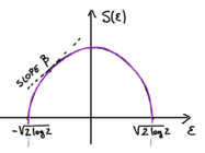
In this problem we study the number ${\mathcal {N}}(E)dE$ of configurations having energy $E_{\alpha }\in [E,E+dE]$. This quantity is a random variable, for large $N$, we will show that its typical value scales as

${\mathcal {N}}(E)=e^{N\Sigma \left({\frac {E}{N}}\right)+o(N)},\quad \quad \Sigma (\epsilon )={\begin{cases}\log 2-\epsilon ^{2}\quad &{\text{ if }}|\epsilon |\leq {\sqrt {\log 2}}\\0\quad &{\text{ if }}|\epsilon |>{\sqrt {\log 2}}\end{cases}}$

The function $\Sigma (\epsilon )$ is the entropy of the model (see sketch). The point where the entropy vanishes, $\epsilon =-{\sqrt {\log 2}}$, is the energy density of the ground state, consistently with what we obtained in the lecture. The entropy is maximal at $\epsilon =0$: the highest number of configurations have vanishing energy density.

1. Averages: the annealed entropy. We begin by computing the “annealed" entropy $\Sigma ^{A}$, which is the function that controls the behaviour of the average number of configurations at a given energy, ${\overline {{\mathcal {N}}(E)}}={\text{exp}}\left(N\Sigma ^{A}\left({\frac {E}{N}}\right)+o(N)\right)$. Compute this function using the representation ${\mathcal {N}}(E)dE=\sum _{\alpha =1}^{2^{N}}\chi _{\alpha }(E)dE\;$ [with $\chi _{\alpha }(E)=1$ if $E_{\alpha }\in [E,E+dE]$ and $\chi _{\alpha }(E)=0$ otherwise], together with the distribution $p(E)$ of the energies of the REM configurations. When does $\Sigma ^{A}$ coincide with the entropy defined above (which we define as the “quenched” entropy in the following)?

2. Self-averaging. For $|\epsilon |\leq {\sqrt {\log 2}}$ the quantity ${\mathcal {N}}$ is self-averaging: its distribution concentrates around the average value ${\overline {\mathcal {N}}}$ when $N\to \infty$. Show that this is the case by computing the second moment ${\overline {{\mathcal {N}}^{2}}}$ and using the central limit theorem. Show that this is no longer true in the region where the annealed entropy is negative: why does one expect fluctuations to be relevant in this region?

3. Rare events vs typical values. For $|\epsilon |>{\sqrt {\log 2}}$ the annealed entropy is negative: the average number of configurations with those energy densities is exponentially small in $N$. This implies that the probability to get configurations with those energy is exponentially small in $N$: these configurations are rare. Do you have an idea of how to show this, using the expression for ${\overline {\mathcal {N}}}$? What is the typical value of ${\mathcal {N}}$ in this region? Justify why the point where the entropy vanishes coincides with the ground state energy of the model.

Comment: this analysis of the landscape suggests that in the large $N$ limit, the fluctuations due to the randomness become relevant when one looks at the bottom of their energy landscape, close to the ground state energy density. We show below that this intuition is correct, and corresponds to the fact that the partition function $Z$ has an interesting behaviour at low temperature.

Problem 1.2: the free energy and the freezing transition

We now compute the equilibrium phase diagram of the model, and in particular the quenched free energy density $f$ which controls the scaling of the typical value of the partition function, $Z\sim e^{-N\beta \,f+o(N)}$. We show that the free energy equals to

$f={\begin{cases}&-\left(T\log 2+{\frac {1}{4T}}\right)\quad {\text{if}}\quad T\geq T_{c}\\&-{\sqrt {\log 2}}\quad {\text{if}}\quad T<T_{c}\end{cases}}\quad \quad T_{c}={\frac {1}{2{\sqrt {\log 2}}}}.$

At $T_{c}$ a transition occurs, often called freezing transition: in the whole low-temperature phase, the free-energy is “frozen” at the value that it has at the critical temperature $T=T_{c}$.

1. The thermodynamical transition and the freezing. The partition function the REM reads $Z=\sum _{\alpha =1}^{2^{N}}e^{-\beta E_{\alpha }}=\int dE\,{\mathcal {N}}(E)e^{-\beta E}.$ Using the behaviour of the typical value of ${\mathcal {N}}$ determined in Problem 1, derive the free energy of the model (hint: perform a saddle point calculation). What is the order of this thermodynamic transition?

2. Entropy. What happens to the entropy of the model when the critical temperature is reached, and in the low temperature phase? What does this imply for the partition function $Z$?

3. Fluctuations, and back to average vs typical. Similarly to what we did for the entropy, one can define an annealed free energy $f^{A}$ from ${\overline {Z}}=e^{-N\beta f^{A}+o(N)}$: show that in the whole low-temperature phase this is smaller than the quenched free energy obtained above. Putting all the results together, justify why the average of the partition function in the low-T phase is "dominated by rare events".

Comment: the low-T phase of the REM is a frozen phase, characterized by the fact that the free energy is temperature independent, and that the typical value of the partition function is very different from the average value. In fact, the low-T phase is also <emph> a glass phase </emph> in the sense discussed in the lecture. It is characterized by the fact that Replica Symmetry is broken, as one sees explicitly by re-deriving the free energy through the replica method. We go back to this in the next lectures/TDs.