T-I

Goal: derive the equilibrium phase diagram of the simplest spin-glass model, the Random Energy Model (REM).
Techniques: saddle point approximation, Legendre transform, probability theory.

A dictionary for large-N disordered systems

• Exponentially scaling variables. We will consider positive random variables $X_{N}$ which depend on a parameter $N\gg 1$ (the number of degrees of freedom: for a system of size $L$ in dimension $d$, $N=L^{d}$) and which have the scaling $X_{N}\sim e^{NY_{N}}$: this means that the rescaled variable $Y_{N}=N^{-1}\log X_{N}$ has a well defined distribution that remains of $O(1)$ when $N\to \infty$. The standard example we have in mind are the partition functions of disordered systems with $N$ degrees of freedom, $Z_{N}\sim e^{-\beta Nf_{N}}$: here $X_{N}\to Z_{N}$ and $Y_{N}\to -\beta f_{N}$, where $f_{N}$ is the free energy density. Let $P_{X_{N}}(x),P_{Y_{N}}(y)$ be the distributions of $X_{N}$ and $Y_{N}$.


• Self-averaging. A random variable $Y_{N}$ is self-averaging when, in the limit $N\to \infty$, its distribution concentrates around the average, collapsing to a deterministic value:

  $\lim _{N\to \infty }Y_{N}=\lim _{N\to \infty }{\overline {Y_{N}}}\equiv {\overline {Y_{\infty }}}.$

  This happens when its fluctuations are small compared to the average, meaning that ^[*]

  $\lim _{N\to \infty }{\frac {\overline {Y_{N}^{2}}}{{\overline {Y_{N}}}^{2}}}=1.$

  When the random variable is not self-averaging, it remains distributed in the limit $N\to \infty$. When it is self-averaging, sample-to-sample fluctuations are suppressed when $N$ is large. This property holds for the free energy of all the disordered systems we will consider. This is very important property: it implies that the free energy (and therefore all the thermodynamics observables, that can be obtained taking derivatives of the free energy) does not fluctuate from sample to sample when $N$ is large, and so the physics of the system does not depend on the particular sample. Notice that while intensive quantities like $Y_{N}$ (like the free energy density) are self-averaging, quantities scaling exponentially like $X_{N}$ (like the partition function) are not necessarily so, see below.



• Average and typical. The typical value of a random variable is the value at which its distribution peaks (it is the most probable value). For self-averaging quantities, in the limit $N\to \infty$ average and typical value coincide. In general, it might not be so!


We discuss an example to fix the ideas. Often, quantities like $Y_{N}$ have a distribution that for large $N$ takes the form $P_{Y_{N}}(y)\sim e^{-N^{\omega }g(y)+{\text{subleading}}}$ where $g(y)$ is some positive function and $\omega >0$. This is called a large deviation form for the probability distribution, with speed $N^{\omega }$. This distribution is of $O(1)$ for the value $y^{\text{typ}}$ such that $g(y^{\text{typ}})=0=g'(y^{\text{typ}})$: this value is the typical value of $Y_{N}$ (asymptotically at large $N$); all the other values of $y$ are associated to a probability that is exponentially small in $N^{\omega }$: they are exponentially rare. Consider now an exponentially scaling quantity like $X_{N}=e^{NY_{N}}$, and let’s fix $\omega =1$. The asymptotic typical values $x^{\text{typ}}$ and $y^{\text{typ}}$ are related by: $y^{\text{typ}}=\lim _{N\to \infty }{\frac {\log x^{\text{typ}}}{N}},$

so the scaling of $x^{\text{typ}}$ is $x^{\text{typ}}\sim e^{Ny^{\text{typ}}}$. Let us now look at the scaling of the average. The average of $X_{N}$ can be computed with the saddle point approximation for large $N$:

${\overline {X_{N}}}=\int dy\,P_{Y_{N}}(y)\,e^{Ny}=\int dy\,e^{N[y-g(y)]+o(N)}=e^{N[y^{*}-g(y*)]+o(N)},$

where $y^{*}$ is the point maximising the shifted function ${\tilde {g}}(y)=y-g(y)$. In this example, $y^{*}\neq y^{\text{ty}}$: the asymptotic of the average value of $X_{N}$ is different from the asymptotic of the typical value. In particular, the average is dominated by rare events, i.e. realisations in which $Y_{N}$ takes the value $y^{*}$, whose probability of occurrence is exponentially small.




• Quenched averages. Let us go back to $X_{N}$: how to get $y^{\text{typ}}$ from it? When $Y_{N}$ is self-averaging, $y^{\text{typ}}=\lim _{N\to \infty }{\overline {Y_{N}}}=\lim _{N\to \infty }{\frac {\overline {\log X_{N}}}{N}}\equiv \lim _{N\to \infty }{\frac {\log x^{\text{typ}}}{N}}$

  where in the last line we have used that $y^{\text{typ}}=\lim _{N\to \infty }N^{-1}\log x_{N}^{\text{typ}}$.

  In the language of disordered systems, computing the typical value of $X_{N}$ through the average of its logarithm corresponds to performing a quenched average: from this average, one extracts the correct asymptotic value of the self-averaging quantity $Y_{N}$.


• Annealed averages. The quenched average does not necessarily coincide with the annealed average, defined as:

  $y_{\text{a}}=\lim _{N\to \infty }{\frac {\log {\overline {X_{N}}}}{N}}.$

  In fact, it always holds ${\overline {\log X_{N}}}\leq \log {\overline {X_{N}}}$ because of the concavity of the logarithm. When the inequality is strict and quenched and annealed averages are not the same, it means that $X_{N}$ is not self-averaging, and its average value is exponentially larger than the typical value (because the average is dominated by rare events). In this case, to get the correct limit of the self-averaging quantity $Y_{N}$ one has to perform the quenched average.^[**] This is what happens in the glassy phases discussed in these TDs.

[*] - See here for a note on the equivalence of these two criteria.

[**] - Notice that the opposite is not true: one can have situations in which the partition function is not self-averaging, but still the quenched free energy coincides with the annealed one.

Problems

These problems deal with the Random Energy Model (REM). The REM has been introduced in ^[1] . In the REM the system can take $2^{N}$ configurations ${\vec {\sigma }}^{\alpha }=(\sigma _{1}^{\alpha },\cdots ,\sigma _{N}^{\alpha })$ with $\sigma _{i}^{\alpha }=\pm 1$. To each configuration $\alpha =1,\cdots ,2^{N}$ is assigned a random energy $E_{\alpha }$. The random energies are independent, taken from a Gaussian distribution $p(E)=(2\pi N)^{-1/2}e^{-{\frac {E^{2}}{2N}}}.$

Problem 1.1: the energy landscape of the REM

Entropy of the Random Energy Model

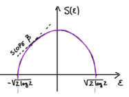
In this problem we study the random variable ${\mathcal {N}}(E)dE$, that is the number of configurations having energy $E_{\alpha }\in [E,E+dE]$. For large $N$ this variable scales as ${\mathcal {N}}(E)=e^{NS\left(E/N\right)+o(N)}$. Let $\epsilon =E/N$. We show that the typical value of $S(\epsilon )$, the quenched entropy density of the model (see sketch), is given by:

$S(\epsilon )={\begin{cases}\log 2-{\frac {\epsilon ^{2}}{2}}\quad &{\text{ if }}|\epsilon |\leq {\sqrt {2\,\log 2}}\\0\quad &{\text{ if }}|\epsilon |>{\sqrt {2\,\log 2}}\end{cases}}$

The point where the entropy vanishes, $\epsilon =-{\sqrt {2\,\log 2}}$, is the energy density of the ground state. The entropy is maximal at $\epsilon =0$: the highest number of configurations have vanishing energy density.

1. Averages: the annealed entropy. We begin by computing the annealed entropy $S_{\text{a}}$, which is defined by the average ${\overline {{\mathcal {N}}(E)}}={\text{exp}}\left(NS_{\text{a}}\left(E/N\right)+o(N)\right)$. Compute this function using the representation ${\mathcal {N}}(E)dE=\sum _{\alpha =1}^{2^{N}}\chi _{\alpha }(E)dE\;$ [with $\chi _{\alpha }(E)=1$ if $E_{\alpha }\in [E,E+dE]$ and $\chi _{\alpha }(E)=0$ otherwise].

2. Self-averaging. For $|\epsilon |\leq {\sqrt {2\,\log 2}}$ the quantity ${\mathcal {N}}$ is self-averaging: its distribution concentrates around the average value ${\overline {\mathcal {N}}}$ when $N\to \infty$. Show this by computing the second moment ${\overline {{\mathcal {N}}^{2}}}$. Deduce that $S(\epsilon )=S_{a}(\epsilon )$ when $|\epsilon |\leq {\sqrt {2\,\log 2}}$. This property of being self-averaging is no longer true in the region where the annealed entropy is negative: why does one expect fluctuations to be relevant in this region?

3. Rare events. For $|\epsilon |>{\sqrt {2\,\log 2}}$ the annealed entropy is negative: the average number of configurations with those energy densities is exponentially small in $N$. This implies that the probability to get configurations with those energy is exponentially small in $N$: these configurations are rare. Do you have an idea of how to show this, using the expression for ${\overline {\mathcal {N}}}?$ What is the typical value of ${\mathcal {N}}$ in this region? Putting everything together, derive the form of the typical value of the entropy density. Why the point where the entropy vanishes coincides with the ground state energy of the model?

Check out: key concepts

Self-averaging, average value vs typical value, large deviations, rare events, saddle point approximation, freezing transition, overlap distribution.

To know more

• Derrida. Random-energy model: limit of a family of disordered models [1]

• A note on terminology:

The terms “quenched” and “annealed” come from metallurgy and refer to the procedure in which you cool a very hot piece of metal: a system is quenched if it is cooled very rapidly (istantaneously changing its environment by putting it into cold water, for instance) and has to adjusts to this new fixed environment; annealed if it is cooled slowly, kept in (quasi)equilibrium with its changing environment at all times. Think now at how you compute the free energy, and at disorder as the environment. In the quenched protocol, you compute the average over configurations of the system keeping the disorder (environment) fixed, so the configurations have to adjust to the given disorder. Then you take the log and only afterwards average over the randomness (not even needed, at large $N$, if the free-energy is self-averaging). In the annealed protocol instead, the disorder (environment) and the configurations are treated on the same footing and adjust to each others, you average over both simultaneously.